Python-大数据分析之常用库

1. 数据采集与第三方数据接入

1-1. Beautiful Soup

Beautiful Soup 是一个用于解析HTML和XML文档的库，非常适用于网页爬虫和数据抓取。可以提取所需信息，无需手动分析网页源代码，简化了从网页中提取数据的过程，使得数据抽取变得更加容易。

应用场景
- 网络爬虫： 用于从网页中抓取所需数据。
- 数据抽取： 从HTML文档中提取数据并进行分析。
- 数据清洗： 帮助清理和规范不一致的HTML数据。

功能特点
- 解析器灵活性： Beautiful Soup支持多种解析器，如Python的内置解析器（html.parser）、lxml解析器（需要安装lxml库）以及html5lib（需要安装html5lib库）。
- 方便的遍历方法： 可以遍历文档树、搜索特定元素、提取数据。
- 容错能力强： 能够处理“糟糕”的HTML代码，修复标记不完整的标签等问题，让解析过程更加稳定。
- 支持编码转换： 可以自动识别文档编码，或者手动指定编码进行解析。

基本用法

解析器初始化： 通过将HTML文档传递给Beautiful Soup来创建解析器对象。


from bs4 import BeautifulSoup
# 从文件中读取HTML
with open("example.html", "r") as file:
    soup = BeautifulSoup(file, "html.parser")

遍历文档树： 可以使用标签名称、类名、id等属性进行文档元素的遍历和搜索。


x
# 通过标签名获取元素
title = soup.title

# 通过类名获取元素
important_texts = soup.find_all("p", class_="important")

# 通过id获取元素
content = soup.find(id="content")

提取数据： 可以获取元素的文本内容、属性等信息。


xxxxxxxxxx
# 获取文本内容
print(title.text)

# 获取属性值
print(content["href"])

修改文档树： 可以添加、删除或修改文档中的标签和内容。


xxxxxxxxxx
# 创建新的标签
new_tag = soup.new_tag("a", href="http://example.com")
new_tag.string = "Link Text"

# 在文档中插入新标签
content.append(new_tag)

1-2. Requests

需要与网络交互时，Requests库是不可或缺。Requests简化了与目标网站接口的通信，易于使用且功能强大，支持多种HTTP方法和参数设置，能够轻松发送HTTP请求并处理响应。网络爬虫、API调用或是测试网站，Requests都能够让这些任务变得轻而易举。

在企业数据采购中，经常需要与供应商或合作伙伴的API进行数据交换。使用requests库可以轻松实现数据的发送和接收，无论是从外部API获取数据还是向外部API推送数据，都可以通过requests来完成。

Requests库特点
- 简单易用： Requests提供了简洁的API，使得发送HTTP请求变得非常简单。
- 多种HTTP方法支持： 支持GET、POST、PUT、DELETE等HTTP方法。
- 自动解析： 能够自动解析JSON响应和处理URL编码等。
- Session支持： 可以创建持久性会话，保持会话状态，方便维护会话信息。
- SSL证书验证、Cookie支持、重定向等： 提供了多种功能以处理各种HTTP请求和响应情况。

基本用法

发送GET请求：通过向外部API发送GET请求来获取数据（获取外部数据源）


xxxxxxxxxx
# API数据获取
import requests

response = requests.get('https://api.openweathermap.org/data/2.5/weather?q=London&appid=your_api_key')
if response.status_code == 200:
    weather_data = response.json()
    # 处理数据逻辑

    
# Web数据抓取 
import requests
from bs4 import BeautifulSoup

response = requests.get('https://example.com')
if response.status_code == 200:
    soup = BeautifulSoup(response.text, 'html.parser')
    # 提取所需数据信息

发送POST请求：使用POST请求向外部API发送数据（推送数据给外部接口）


xxxxxxxxxx
import requests

payload = {'key1': 'value1', 'key2': 'value2'}
headers = {'Content-Type': 'application/json', 'Authorization': 'Bearer YOUR_TOKEN'}

response = requests.post('https://api.example.com/endpoint', json=payload, headers=headers)
if response.status_code == 201:
    # 处理成功发送数据后的响应

错误处理与异常情况：


xxxxxxxxxx
import requests

try:
    response = requests.get('https://api.example.com/data')
    response.raise_for_status()  # 如果响应状态码不是200，则会抛出HTTPError异常
    data = response.json()
    # 处理数据
except requests.HTTPError as http_err:
    print(f'HTTP error occurred: {http_err}')
except Exception as err:
    print(f'Other error occurred: {err}')

使用Session保持会话：


xxxxxxxxxx
with requests.Session() as session:
    session.get('https://example.com/login', auth=('user', 'pass'))
    # 保持登录状态进行后续请求
    response = session.get('https://example.com/dashboard')

处理认证和权限


xxxxxxxxxx
# Token认证：使用请求头中的Token进行认证
headers = {'Authorization': 'Bearer YOUR_TOKEN'}

# Basic Auth：通过提供用户名和密码进行基本认证。
auth = ('username', 'password')
response = requests.get('https://api.example.com/data', auth=auth)

日志记录与监控


xxxxxxxxxx
import requests
import logging

logging.basicConfig(filename='requests.log', level=logging.INFO)

try:
    response = requests.get('https://api.example.com/data')
    response.raise_for_status()
    logging.info('Request successful')
except requests.HTTPError as http_err:
    logging.error(f'HTTP error occurred: {http_err}')
except Exception as err:
    logging.error(f'Other error occurred: {err}')

1-3. Beautiful Soup与Requests总结对比

特点	Beautiful Soup	Requests
主要功能	解析HTML和XML文档，提取数据	发送HTTP请求，处理响应
用途	网页解析、数据抽取和处理	向服务器发起HTTP请求、处理响应，获取网络数据
关注重点	文档解析、数据提取	HTTP请求和响应的处理
主要特点	- 提供多种解析器 - 方便的API来遍历文档树、搜索元素、提取数据 - 修复HTML不完整标签	- 提供简洁的API - 支持多种HTTP方法 - 处理认证、Cookie、SSL验证等
适用场景	从网页中提取特定数据、数据清洗、提取链接等	发送HTTP请求、获取网页内容、与API进行交互

2. 数据分析

2-1. Jupyter Notebook

Jupyter Notebook是一个开源的交互式笔记本环境，支持多种编程语言，最常用的是Python。它以网页的形式提供一个交互式界面，允许用户在浏览器中编写和运行代码、展示文本、图像、公式等内容，并保存成为具有可执行代码、可视化结果和解释性文档的笔记本。Jupyter Notebook是数据科学家和研究人员的最爱，无论是在进行数据分析、机器学习建模还是原型设计，Jupyter Notebook都是无可替代的工具。

Jupyter Notebook作为一个灵活、交互式、功能丰富的工具，为数据科学家、教育工作者和开发人员提供了一个方便的平台，可以方便地探索数据、编写文档和演示成果。

主要特点和功能
- 多语言支持： Jupyter支持多种编程语言，如Python、R、Julia等，通过内核系统可以轻松切换语言。
- 交互式运行： 可以分段执行代码，实时查看输出结果，有助于探索数据和算法。
- 富文本展示： 支持Markdown、LaTeX等富文本格式，可以插入文本、图像、公式、超链接等。
- 数据可视化： 可以直接在Notebook中绘制图表、图像等可视化结果，并与代码交互。
- 方便共享： 笔记本可以导出成HTML、PDF、Markdown等格式，方便分享和展示成果。
- 支持扩展： 有丰富的插件和扩展功能，可以增强编辑和运行环境。
用途和应用场景
- 数据分析和可视化： 在数据科学领域广泛应用，用于数据清洗、探索、分析和可视化。
- 教学和学习： 作为教学工具，可以编写教程、示例代码，并直观地展示结果，有助于学习和教学。
- 实验和原型开发： 用于快速原型设计和实验，探索算法、库和新技术。
- 文档编写： 用于编写技术文档、报告和演示文稿，结合代码和解释性文本。

使用方法
- 安装Jupyter Notebook： 通过pip或conda安装Jupyter Notebook。
- 启动Jupyter Notebook： 在命令行中输入jupyter notebook，会在浏览器中打开Jupyter界面。
- 创建和编辑笔记本： 在界面中新建Notebook文件，选择所需编程语言的内核，开始编写和运行代码。
- 编辑和运行代码： 将代码写入单元格，按下Shift+Enter执行单元格中的代码，并查看输出结果。
- 添加文本和图像： 使用Markdown语法添加文本、标题、图像等丰富的内容。
- 保存和分享： 可以保存笔记本为.ipynb文件，也可以导出成其他格式用于分享。

2-2. NumPy

NumPy是Python中用于科学计算的一个强大的库，主要用于处理数组和矩阵运算。它提供了丰富的功能和高效的数据结构，是许多科学和工程领域中常用的核心库之一。

主要特点和功能
- 多维数组对象： 提供了ndarray对象，用于表示多维数组，可以进行高效的数值运算。
- 数学函数： 包括线性代数、傅立叶变换、随机数生成等丰富的数学函数和工具。
- 广播功能： 能够处理不同形状的数组，自动执行元素级运算，极大地简化了代码编写。
- 性能优化： NumPy底层使用C语言编写，操作数组的运算速度非常快，是因为它具有优化的算法和数据结构。
- 与其他工具集成： 可以与其他工具（如Pandas、Matplotlib等）良好集成，为数据分析和可视化提供基础支持。
用途和应用场景
- 数据处理和分析： 在数据科学领域中，NumPy常用于处理、转换和分析数据，尤其是大量数据的计算。
- 科学计算： 在科学计算、工程领域，例如物理学、生物学、金融学等领域，用于模拟、分析和解决数学问题。
- 机器学习和人工智能： 在机器学习领域，NumPy用于处理和转换数据，作为许多机器学习算法的基础。
- 图像处理： 在图像处理和计算机视觉中，NumPy提供了对图像数据进行处理和操作的功能。

基本用法示例

NumPy使用介绍可见另一篇博客文章：https://blog.csdn.net/wt334502157/article/details/128185332

2-3. pandas

Pandas是Python中用于数据处理和分析的强大库，它建立在NumPy的基础上，提供了更高级的数据结构和工具，使得数据操作更加便捷和高效。Pandas通常用于处理结构化数据，比如表格数据、时间序列等，无论是需要进行数据清洗、转换还是统计分析，Pandas都可以帮助您快速达成目标

主要特点和功能
- DataFrame对象： 提供了DataFrame对象，类似于电子表格或SQL数据库中的表格，用于处理二维数据。
- Series对象： 提供了Series对象，类似于一维数组或列表，用于处理一维数据。
- 数据对齐和处理： 能够轻松处理缺失数据、重复数据、数据合并、数据对齐等操作。
- 灵活的数据操作： 支持数据的切片、筛选、聚合、分组等操作，操作更简单直观。
- 数据读写： 支持多种数据格式的读写，如CSV、Excel、SQL、JSON等。
- 数据可视化： 集成了Matplotlib等库，能够进行数据可视化和绘图操作。
用途和应用场景
- 数据清洗和预处理： 用于处理和清洗数据，包括缺失值处理、数据转换、数据规范化等。
- 数据分析和探索： 在数据科学领域中，用于数据探索、统计分析、建模等。
- 时间序列处理： 用于处理时间序列数据，如金融数据、传感器数据等。
- 数据可视化： 可以配合Matplotlib等库进行数据可视化，绘制图表和图形。

基本用法示例

Pandas使用介绍可见另一篇博客文章：https://blog.csdn.net/wt334502157/article/details/128219770

3. 数据展示

3-1. matplotlib

Matplotlib是Python中用于绘制图表和可视化数据的库，是Python中最常用的数据可视化库之一，无论是在制作科学图表、数据可视化还是报告，都具有高度的可定制性，Matplotlib提供了丰富的绘图选项，可以让数据以最吸引人的方式呈现。

主要特点和功能
- 各种图表类型： 支持线图、柱状图、散点图、饼图、直方图、等高线图等多种类型的图表。
- 高度可定制： 用户可以对图表的各种属性进行自定义，包括颜色、线型、标签、标题等。
- 支持多种输出格式： 可以生成图像并保存为多种格式，如PNG、JPG、SVG、PDF等。
- 交互式功能： 结合Jupyter Notebook等环境可以实现交互式图表展示。
- 与Pandas集成： 可以方便地与Pandas等库结合使用，直接绘制DataFrame中的数据。
用途和应用场景
- 数据可视化： 在数据科学和数据分析中广泛应用，用于展示和传达数据分析的结果。
- 科学研究： 在科学研究中用于绘制实验数据、模拟结果和科学图表。
- 工程和统计分析： 用于制作工程图、统计图和报告图表。
- 教学和学习： 作为教学工具，用于制作教程、教材以及演示。

基本用法示例
1. 绘制折线图：


xxxxxxxxxx
import matplotlib.pyplot as plt

x = [1, 2, 3, 4, 5]
y = [2, 4, 6, 8, 10]

plt.plot(x, y)
plt.xlabel('X Axis')
plt.ylabel('Y Axis')
plt.title('Line Chart')
plt.show()

绘制柱状图：


xxxxxxxxxx
import matplotlib.pyplot as plt

x = ['板甲', '锁甲', '皮甲', '布甲']
y = [30, 12, 37, 26]

plt.bar(x, y)
plt.xlabel('装备类型')
plt.ylabel('玩家占比')
plt.title('各甲玩家占比')
# Windows 设置显示中文
plt.rcParams['font.sans-serif'] = 'SimHei'
plt.show()

绘制散点图：


xxxxxxxxxx
import matplotlib.pyplot as plt

x = [1, 2, 3, 4, 5]
y = [2, 2, 6, 9, 16]

plt.scatter(x, y)
plt.xlabel('X Axis')
plt.ylabel('Y Axis')
plt.title('Scatter Plot')
plt.show()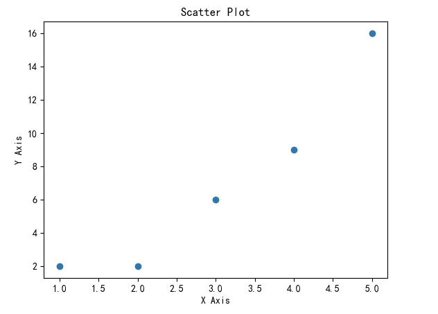

绘制雷达图


xxxxxxxxxx
import numpy as np
import matplotlib.pyplot as plt
# 创建figure
fig = plt.figure(dpi=120)
# 准备好极坐标系的数据
# 半径为[0,1]
r = np.arange(0, 1, 0.001)
theta = 2 * 2*np.pi * r
# 极坐标下绘制
line, = plt.polar(theta, r, color='#ee8d18', lw=3)
plt.show()

4. 机器学习

4-1. seaborn

Seaborn是建立在Matplotlib之上的数据可视化库，专注于创建具有统计意义的各种图表。它提供了简单的高级接口，可以轻松地创建漂亮的统计图表，并且具有更好的默认设置，使得数据可视化变得更加简单和直观。

Seaborn提供了一些Matplotlib不提供或不易实现的高级图表类型，如小提琴图、热图、分布图等，这些图表类型能更好地展示数据的分布、关系和特征；具有更好看的默认主题和调色板，使得图表外观更为美观，无需额外调整，让用户在默认情况下就能得到具有吸引力的图表。

虽然Seaborn更加强大，但并不是取代Matplotlib，而是在Matplotlib的基础上提供了更多的功能和便利性，特别适用于统计分析、数据探索和一些高级的可视化需求。在实际应用中，它们可以结合使用，根据不同的需求选择合适的库来绘制图表。

主要特点和功能：

统计图表： 提供了针对统计分析常用的图表类型，如箱线图、小提琴图、热图、聚类图等。
内置主题和调色板： 具有美观的默认主题和调色板，使得图表的外观更加吸引人。
数据探索和分析： 支持对数据集的直观探索，可用于探索数据的分布、关系等。
与Pandas集成： 能够方便地与Pandas等库结合使用，直接绘制DataFrame中的数据。
多变量图表： 支持绘制多变量之间的关系图、热图等复杂图表。

用途和应用场景：

数据探索和分析： 在数据科学领域中广泛应用，用于数据探索、可视化数据分布、关系等。
统计分析报告： 用于生成漂亮的图表，加入报告和论文中，提供直观的数据支持。
数据可视化： 作为Matplotlib的补充，提供更高级、更美观的图表，适用于各种数据可视化需求。

基本用法示例：

绘制箱线图：


xxxxxxxxxx
import seaborn as sns
import matplotlib.pyplot as plt

# 加载示例数据集
tips = sns.load_dataset("tips")

sns.boxplot(x="day", y="total_bill", data=tips)
plt.xlabel('日期')
plt.ylabel('账单')
plt.title('每日总账单方框图')
# Windows 设置显示中文
plt.rcParams['font.sans-serif'] = 'SimHei'
plt.show()

绘制小提琴图：


xxxxxxxxxx
import seaborn as sns
import matplotlib.pyplot as plt

# 加载示例数据集
tips = sns.load_dataset("tips")

sns.violinplot(x="day", y="total_bill", data=tips)
plt.xlabel('日期')
plt.ylabel('账单')
plt.title('每日总账单小提琴图图')
# Windows 设置显示中文
plt.rcParams['font.sans-serif'] = 'SimHei'
plt.show()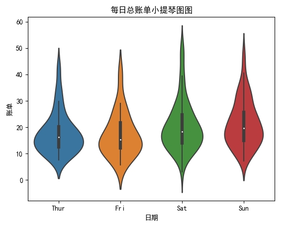

绘制热图：


xxxxxxxxxx
import seaborn as sns
import matplotlib.pyplot as plt

# 创建一个矩阵数据
data = sns.load_dataset("flights").pivot("month", "year", "passengers")

sns.heatmap(data, annot=True, fmt="d", cmap="YlGnBu")
plt.xlabel('年')
plt.ylabel('月')
plt.title('航班乘客热呈图')
plt.show()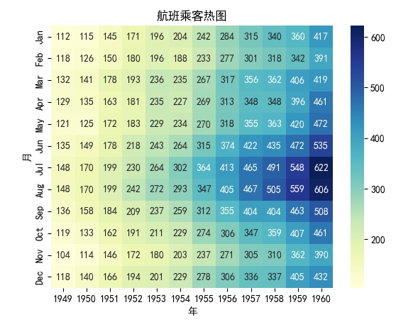

4-2. scikit-learn

scikit-learn（sklearn）是一个用于机器学习和数据挖掘的Python库，提供了各种机器学习算法实现和简单而有效的工具，用于数据挖掘和数据分析。它建立在NumPy、SciPy和Matplotlib之上，包含了各种机器学习算法和工具，适用于各种机器学习任务。

主要特点和功能

丰富的机器学习算法： 包含了许多常用的监督学习和无监督学习算法，如回归、分类、聚类、降维等。
易于使用的API： 具有统一和一致的API，使得用户可以方便地实现各种机器学习算法。
数据预处理和特征工程： 提供了数据预处理、特征选择、特征提取等功能，用于准备数据以供模型训练。
模型评估和验证： 提供了各种评估指标和验证方法，用于评估模型的性能和泛化能力。
与其他库的集成： 可以与NumPy、Pandas等库无缝集成，方便处理和转换数据。
可扩展性和灵活性： 支持模型的扩展和自定义，用户可以方便地实现自定义的机器学习算法。

常见的机器学习任务
- 分类： 区分数据点属于哪个类别，如垃圾邮件分类、图像识别等。
- 回归： 预测数值型数据，如房价预测、股票价格预测等。
- 聚类： 将数据分成不同的组别，发现数据中的模式，如用户分群、市场细分等。
- 降维： 减少数据集维度，保留主要特征，如图像处理、文本挖掘等。

基本用法示例
1. 简单的线性回归示例


xxxxxxxxxx
from sklearn.linear_model import LinearRegression
from sklearn.datasets import make_regression
from sklearn.model_selection import train_test_split
from sklearn.metrics import mean_squared_error
import matplotlib.pyplot as plt

# 设置中文字体以支持中文显示
plt.rcParams['font.sans-serif'] = ['SimHei']
plt.rcParams['axes.unicode_minus'] = False

# 生成随机回归数据集
X, y = make_regression(n_samples=100, n_features=1, noise=20, random_state=42)

# 划分数据集
X_train, X_test, y_train, y_test = train_test_split(X, y, test_size=0.3, random_state=42)

# 创建线性回归模型并拟合数据
model = LinearRegression()
model.fit(X_train, y_train)

# 预测并评估模型
y_pred = model.predict(X_test)
mse = mean_squared_error(y_test, y_pred)
print("均方误差:", mse)

# 可视化结果
plt.scatter(X_test, y_test, color='black')
plt.plot(X_test, y_pred, color='blue', linewidth=3)
plt.xlabel('X')
plt.ylabel('y')
plt.title('线性回归')
plt.show()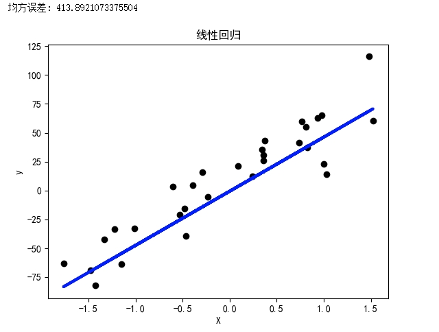

K-Means聚类示例


xxxxxxxxxx
from sklearn.datasets import make_blobs
from sklearn.cluster import KMeans
import matplotlib.pyplot as plt

# 设置中文字体以支持中文显示
plt.rcParams['font.sans-serif'] = ['SimHei']
plt.rcParams['axes.unicode_minus'] = False

# 生成随机聚类数据
X, _ = make_blobs(n_samples=300, centers=4, cluster_std=0.60, random_state=42)

# 构建并拟合K-Means模型
kmeans = KMeans(n_clusters=4)
kmeans.fit(X)

# 可视化聚类结果
plt.scatter(X[:, 0], X[:, 1], c=kmeans.labels_, cmap='viridis')
plt.scatter(kmeans.cluster_centers_[:, 0], kmeans.cluster_centers_[:, 1], s=300, c='red', marker='*', label='聚类中心')
plt.title('K-Means聚类')
plt.legend()
plt.show()

决策树分类示例


xxxxxxxxxx
from sklearn.datasets import load_iris
from sklearn.tree import DecisionTreeClassifier
from sklearn.model_selection import train_test_split
from sklearn.metrics import accuracy_score
from sklearn.tree import plot_tree

# 设置中文字体以支持中文显示
plt.rcParams['font.sans-serif'] = ['SimHei']
plt.rcParams['axes.unicode_minus'] = False

# 加载鸢尾花数据集
iris = load_iris()
X, y = iris.data, iris.target

# 划分数据集
X_train, X_test, y_train, y_test = train_test_split(X, y, test_size=0.3, random_state=42)

# 构建并拟合决策树模型
clf = DecisionTreeClassifier(max_depth=3, random_state=42)
clf.fit(X_train, y_train)

# 预测并评估模型
y_pred = clf.predict(X_test)
accuracy = accuracy_score(y_test, y_pred)
print("准确率:", accuracy)

# 可视化决策树
plt.figure(figsize=(12, 8))
plot_tree(clf, feature_names=iris.feature_names, class_names=iris.target_names, filled=True)
plt.show()

工商企业预测年营业额示例

假设我们想要根据企业的注册资本、成立年份、行业等信息来预测企业的年营业额。以下是一个简化的示例


xxxxxxxxxx
import pandas as pd
from sklearn.model_selection import train_test_split
from sklearn.linear_model import LinearRegression
from sklearn.metrics import mean_squared_error
import matplotlib.pyplot as plt
import numpy as np

# 设置中文字体以支持中文显示
plt.rcParams['font.sans-serif'] = ['SimHei']
plt.rcParams['axes.unicode_minus'] = False

# 手动生成示例数据（假设这是一个简化的数据集）
np.random.seed(42)
data = {
    '注册资本': np.random.randint(100, 1000, 50),
    '成立年份': np.random.randint(2000, 2020, 50),
    '行业': np.random.choice(['制造业', '服务业', '零售业'], 50),
    '年营业额': np.random.randint(100000, 1000000, 50)
}

# 创建DataFrame
df = pd.DataFrame(data)

# 对行业进行独热编码
df = pd.get_dummies(df, columns=['行业'])

# 数据预处理，选择特征和目标值
X = df[['注册资本', '成立年份', '行业_制造业', '行业_服务业', '行业_零售业']]
y = df['年营业额']

# 划分数据集
X_train, X_test, y_train, y_test = train_test_split(X, y, test_size=0.2, random_state=42)

# 创建线性回归模型并拟合数据
model = LinearRegression()
model.fit(X_train, y_train)

# 预测并评估模型
y_pred = model.predict(X_test)
mse = mean_squared_error(y_test, y_pred)
print("均方误差:", mse)

# 可视化结果（展示预测值和实际值的对比）
plt.figure(figsize=(8, 6))
plt.plot(range(len(y_pred)), y_pred, label='预测年营业额', marker='o')
plt.plot(range(len(y_test)), y_test, label='实际年营业额', marker='x')
plt.xlabel('样本编号')
plt.ylabel('年营业额')
plt.title('年营业额预测结果')
plt.legend()
plt.show()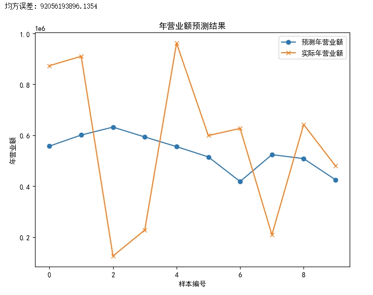

4-3. Keras

Keras 是一个高层神经网络 API，它可以运行在 TensorFlow、Theano 和 Microsoft Cognitive Toolkit（CNTK）之上，使得深度学习任务更加简单和快速。它设计用来快速试验和搭建神经网络模型，具有易用性和灵活性。

主要特点和功能

用户友好性： Keras 提供了简洁一致的 API，易于使用和理解，适合初学者和专业人士。
模块化和可组合性： 允许用户通过堆叠层的方式快速构建神经网络模型，模块化程度高，便于修改和扩展。
支持多种神经网络类型： 支持多种类型的神经网络，包括卷积神经网络（CNN）、循环神经网络（RNN）、深度强化学习等。
灵活性： 可以在 CPU 和 GPU 上无缝运行，支持快速实验和迁移学习。
易于扩展： 可以通过添加自定义层、损失函数、激活函数等来定制模型。
内置高级功能： 提供了各种内置功能，如图像处理、序列处理、优化器、损失函数等。
广泛的社区支持： 拥有庞大的用户社区和开发者支持，提供了丰富的文档和示例。

Keras 的基本用法示例

以下是一个简单的示例，展示了如何使用 Keras 来构建一个简单的全连接神经网络，并训练一个分类模型：


xxxxxxxxxx
import keras
from keras.models import Sequential
from keras.layers import Dense
from keras.optimizers import Adam
from sklearn.datasets import make_classification
from sklearn.model_selection import train_test_split

# 生成分类数据
X, y = make_classification(n_samples=1000, n_features=20, n_classes=2, random_state=42)

# 划分数据集
X_train, X_test, y_train, y_test = train_test_split(X, y, test_size=0.2, random_state=42)

# 创建模型
model = Sequential()
model.add(Dense(64, input_shape=(20,), activation='relu'))
model.add(Dense(32, activation='relu'))
model.add(Dense(1, activation='sigmoid'))

# 编译模型
model.compile(optimizer=Adam(learning_rate=0.001), loss='binary_crossentropy', metrics=['accuracy'])

# 训练模型
history = model.fit(X_train, y_train, batch_size=32, epochs=10, validation_data=(X_test, y_test))

# 可视化训练过程
import matplotlib.pyplot as plt

plt.plot(history.history['accuracy'], label='训练准确率')
plt.plot(history.history['val_accuracy'], label='验证准确率')
plt.xlabel('Epochs')
plt.ylabel('准确率')
plt.legend()
plt.show()

/**
Epoch 1/10
25/25 [====================] - 0s 6ms/step - loss: 0.6231 - accuracy: 0.6900 - val_loss: 0.5630 - val_accuracy: 0.7400
Epoch 2/10
25/25 [====================] - 0s 2ms/step - loss: 0.4710 - accuracy: 0.8525 - val_loss: 0.4817 - val_accuracy: 0.7850
Epoch 3/10
25/25 [====================] - 0s 2ms/step - loss: 0.3752 - accuracy: 0.8763 - val_loss: 0.4277 - val_accuracy: 0.8150
Epoch 4/10
25/25 [====================] - 0s 2ms/step - loss: 0.3247 - accuracy: 0.8925 - val_loss: 0.4103 - val_accuracy: 0.8300
Epoch 5/10
25/25 [====================] - 0s 2ms/step - loss: 0.2992 - accuracy: 0.8950 - val_loss: 0.4085 - val_accuracy: 0.8300
Epoch 6/10
25/25 [====================] - 0s 2ms/step - loss: 0.2821 - accuracy: 0.9025 - val_loss: 0.4048 - val_accuracy: 0.8400
Epoch 7/10
25/25 [====================] - 0s 2ms/step - loss: 0.2696 - accuracy: 0.9038 - val_loss: 0.3964 - val_accuracy: 0.8400
Epoch 8/10
25/25 [====================] - 0s 2ms/step - loss: 0.2598 - accuracy: 0.9025 - val_loss: 0.4061 - val_accuracy: 0.8400
Epoch 9/10
25/25 [====================] - 0s 2ms/step - loss: 0.2484 - accuracy: 0.9150 - val_loss: 0.4035 - val_accuracy: 0.8350
Epoch 10/10
25/25 [====================] - 0s 2ms/step - loss: 0.2383 - accuracy: 0.9125 - val_loss: 0.4063 - val_accuracy: 0.8550
**/